Procedural Space Scene, Part 1: The Sky

I am building Hephaestus, a story-driven anti-4X survival game. The player commands a salvage ark in a hostile arm of the galaxy. The player keeps five thousand cryogenic sleepers alive and decides where the ship goes next.

The game needs a different sky for every star system a campaign visits.

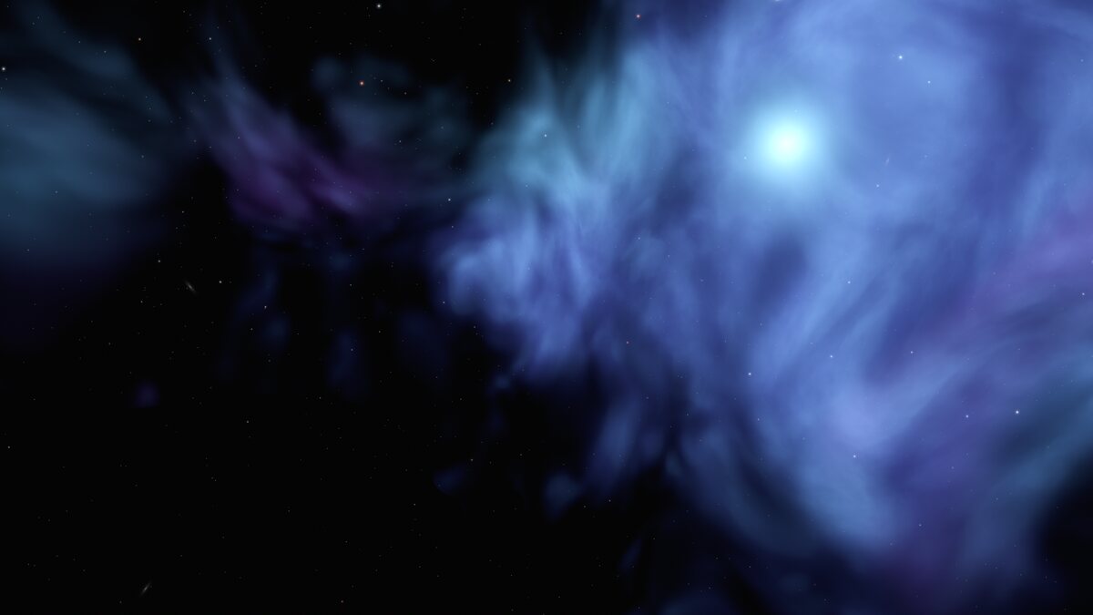Every part of this frame came out of one seed: the nebula, the primary star, the star field and the galaxies behind it.

The backdrop tells the player which system they are in. Each system’s seed generates its own sky, so the view is the one from the ship’s current position.

This part covers the sky only. Planets are the subject of part 2.

Where the idea comes from

This approach is inspired by FTL: Faster Than Light (Subset Games, 2012).

FTL draws the ship in cross-section against a painted backdrop of the current jump destination: a planet, a sun, a nebula, an asteroid field. The backdrop carries no mechanics. It communicates location, and it does that with one composed image per destination.

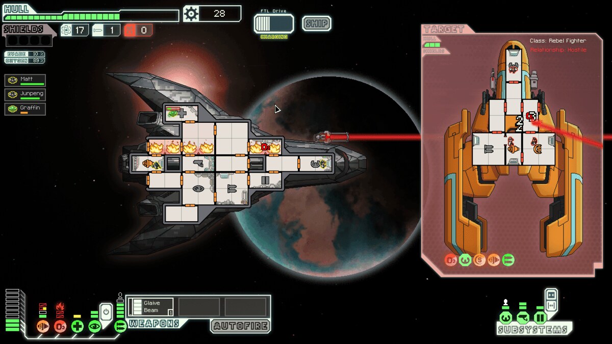FTL: Faster Than Light, Subset Games, 2012. The ship in cross-section, the planet behind it, and every number in the layer on top.

Worth copying:

• The backdrop answers “where am I”, which is a question the player has.
• A small ship against a large environment communicates the premise immediately.
• Every destination arrives as a composed frame, with a subject and somewhere for the eye to go.

The production method does not transfer. FTL’s backdrops are hand-painted, and a run lasts eight sectors, roughly two hours. A Hephaestus campaign runs 250 to 350 turns across hundreds of systems. Hand-painting that many is not practical, and a small repeating set makes the galaxy feel small.

The goal is a generator that produces what FTL’s painters produced.

What the generator has to satisfy

Every system needs its own sky. Not physically distinct, though: two neighbouring systems share almost the same real sky. An astronomically accurate generator produces one image for the whole campaign. The backdrop communicates location, so it differs between locations, and the astronomy is dropped.

The same seed must produce the same sky. The sky is not stored in the save. It is regenerated from the system’s seed every time it is needed, which puts two requirements on it.

Loading a save has to restore the sky the player was looking at. A system also has to look the same on its fiftieth visit as on its first. A place that changes appearance between visits stops reading as a place. Randomness at load time breaks both requirements.

Every sky needs a composition, and content alone will not give it one. A generator that scatters gas evenly across the sphere satisfies every requirement stated so far and produces wallpaper. Each system has to arrive with a subject, somewhere for the eye to go, and somewhere dark for it to read against.

It has to be cheap at runtime. The sky barely moves, so recomputing it every frame is wasted work.

The shape of the answer

Start with the camera, because most of what follows depends on it. It sits at a fixed distance and pivots about the origin inside a cone of roughly eight degrees of yaw and five of pitch. It drifts slowly within that cone so the frame is never completely static, and it never leaves it.

So the sky the player can reach is a small patch of the sphere around them. Call it the reachable cone. It decides the shape of the texture in step 9 and where the billboards go in step 10.

On top of that, four layers:

Layer	What it is	Why it is separate
Nebula	A baked texture covering the reachable cone	Volumetric, expensive, and near enough static
Faint stars	1600 additive billboards on a shell	Point detail a texture cannot keep sharp at every resolution (step 10)
Bright stars	12 billboards with halos	Rare enough that each one is an event
Distant galaxies	10 faint billboards	The universe past this one

The nebula layer carries none of the point detail. Same seed, same crop, with and without the billboards:

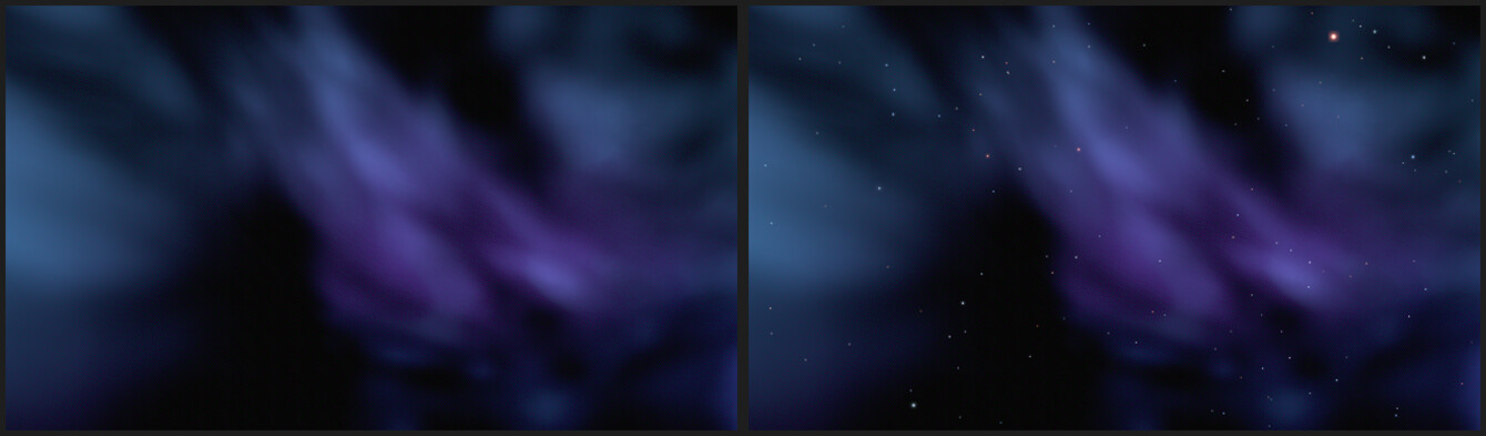One-to-one crops, brightened. Left: the baked nebula on its own. Right: the same frame with the faint stars, bright stars and galaxies drawn over it.

Under all of it, the generator splits into three stages. Keeping them separate is the most useful structural choice in this system.

Where things are. The galactic belt’s axis, the number and size of cloud masses, the position of the primary star. This is composition. It is pure arithmetic on the seed, runs on the CPU, and can be unit tested without a graphics device.

What colour they are. Five colour roles per stellar family: deep shadow, main gas, a contrasting secondary, sparse accents, and hot emissive edges. Plus how much of the sky the gas may occupy. These values are authored in a table rather than derived, so tuning them is a data edit.

What it looks like. Noise, volumetric ray marching, lighting, saturation. This is the expensive part. It runs once on the GPU and is the only part that needs a rendered frame to verify.

The shader never makes decisions that belong to the first two stages. A shader that chooses where a nebula goes has to be run to be understood, which rules out unit tests and diffs.

Step 1: a seed that survives edits

The naive approach breaks determinism as soon as the generator is edited:

var rng := RandomNumberGenerator.new()
rng.seed = campaign_seed
var band_tilt := rng.randf()
var star_angle := rng.randf()
var star_azimuth := rng.randf()

This is deterministic but unmaintainable. Adding one parameter in the middle shifts every draw after it, which changes the sky in every existing save.

The fix is to stop drawing in sequence. Hash the seed together with a named stream instead:

## A stable [0, 1) draw for one named stream of this identity. Streams are spaced
## so that adding a value to one generator never shifts another's draws.
func unit(stream: int) -> float:
	var mixed := StableHash.of_ints(PackedInt64Array([generation_seed, stream]))
	return float(mixed & 0xFF_FFFF) / 16777216.0

Stream identifiers are spaced out, leaving room to add draws inside each one:

const BAND_TILT_STREAM: int = 101
const ANCHOR_COUNT_STREAM: int = 201
const ANCHOR_STREAM: int = 210
const STAR_STREAM: int = 301

The seed itself is a hash of three values. The same system in the same campaign stays stable, and the same campaign seed used by another subsystem does not collide:

generation_seed = StableHash.of_ints(
	PackedInt64Array([
		campaign_seed,
		StableHash.of_string(String(system_id)),
		StableHash.of_string(String(PURPOSE)),
	])
) & StableHash.POSITIVE_MASK

PURPOSE is the literal string presentation.skybox.v1. This lets the campaign seed drive both the terrain generator and the sky without the two producing correlated output.

Step 2: compose along the view axis

The intuitive approach generates the sky uniformly over a sphere, then rotates it until it looks good. That does not work: a rotation can only move content that already exists. It cannot bring a nebula into frame if the generator placed it behind the camera.

So the composition is built around the view axis:

## The direction both presentation cameras look along. They sit above and behind
## the ship, and aim at the origin.
const VIEW_DIRECTION := Vector3(0.0, -0.5285, -0.8489)

Placing anything then reduces to one helper: a direction a given angle from an axis, rolled by a given azimuth. Azimuth zero is screen right for this axis, and a quarter turn is screen down.

static func direction_near_at(axis: Vector3, angle: float, azimuth: float) -> Vector3:
	var tangent := axis.cross(Vector3.UP)
	if tangent.length_squared() < 0.001:
		tangent = axis.cross(Vector3.RIGHT)
	tangent = tangent.normalized()
	var bitangent := axis.cross(tangent).normalized()
	var swing := tangent * cos(azimuth) + bitangent * sin(azimuth)
	return (axis * cos(angle) + swing * sin(angle)).normalized()

Cloud masses are placed in rings measured from that axis. The first ring is close enough to be in frame and far enough out to leave the centre clear:

## The ring of angles off the view axis each anchor may sit in, by index.
const ANCHOR_RINGS: Array[Vector2] = [
	Vector2(0.30, 0.60),   # the subject, always in frame
	Vector2(0.70, 1.20),
	Vector2(1.20, 1.90),
	Vector2(1.80, 2.50),
	Vector2(2.30, 3.00),
]

Those rings, the azimuth rule described next, and a radius per index are the whole anchor placement. Each anchor is packed as xyz direction and w cosine of angular radius. Anchors past the drawn count carry a cosine above one, which the shader reads as switched off:

func cloud_anchors() -> Array[Vector4]:
	var span := MAX_CLOUD_ANCHORS - MIN_CLOUD_ANCHORS + 1
	var drawn := MIN_CLOUD_ANCHORS + int(unit(ANCHOR_COUNT_STREAM) * float(span)) % span
	var anchors: Array[Vector4] = []
	for index: int in range(MAX_CLOUD_ANCHORS):
		if index >= drawn:
			anchors.append(Vector4(0.0, 0.0, 1.0, DISABLED_ANCHOR))
			continue
		var stream := ANCHOR_STREAM + index * 8
		var ring: Vector2 = ANCHOR_RINGS[index]
		# The subject holds the right, so the left stays the darker ground it
		# reads against. A mass that can land anywhere sometimes puts two
		# of them on the same side.
		var azimuth := (
			lerpf(SUBJECT_MIN_AZIMUTH, SUBJECT_MAX_AZIMUTH, unit(stream + 1))
			if index == 0
			else unit(stream + 1) * TAU
		)
		var direction := direction_near_at(
			VIEW_DIRECTION, lerpf(ring.x, ring.y, unit(stream)), azimuth
		)
		var radius_range: Vector2 = ANCHOR_RADII[index]
		var radius := lerpf(radius_range.x, radius_range.y, unit(stream + 2))
		anchors.append(Vector4(direction.x, direction.y, direction.z, cos(radius)))
	return anchors

Only the first anchor gets a constrained azimuth, and that one is the composition: the subject holds one side of the frame so the other stays the darker ground it reads against. Let it land anywhere and some seeds get two competing masses on the same side, and others get nothing to look at. The remaining anchors use the full 360-degree rotation, and act as background depth.

The belt gets the same treatment from the other direction. Its axis is drawn perpendicular to the view direction, so the belt runs across the frame from edge to edge. The axis then tilts slightly to keep the belt off dead centre:

func band_axis() -> Vector3:
	var raw := Vector3(
		float((generation_seed >> 8) & 0xFF) / 127.5 - 1.0,
		float((generation_seed >> 24) & 0xFF) / 127.5 - 1.0,
		float((generation_seed >> 40) & 0xFF) / 127.5 - 1.0,
	)
	if raw.length_squared() <= 0.01:
		raw = Vector3(0.2, 0.8, 0.56)
	var perpendicular := raw - VIEW_DIRECTION * raw.dot(VIEW_DIRECTION)
	if perpendicular.length_squared() <= 0.0001:
		perpendicular = VIEW_DIRECTION.cross(Vector3.UP)
	perpendicular = perpendicular.normalized()
	var tilt := (unit(BAND_TILT_STREAM) * 2.0 - 1.0) * MAX_BAND_TILT
	return (perpendicular * cos(tilt) + VIEW_DIRECTION * sin(tilt)).normalized()

The shader also wants a per-seed offset to push the noise domain around, which is just the seed’s bits spread over three axes:

func shader_offset() -> Vector3:
	return Vector3(
		float(generation_seed & 0xFFFF) / 911.0 + 11.0,
		float((generation_seed >> 16) & 0xFFFF) / 877.0 + 23.0,
		float((generation_seed >> 32) & 0xFFFF) / 853.0 + 37.0,
	)

The camera turns, so the guarantee has to survive turning

The camera moves, so a constraint that only holds at the canonical angle is not worth much. Step 12 shows how far the camera actually drifts, and the test that checks this constraint holds across that drift.

The star sits 16 to 24 degrees off the view axis. Its horizontal offset on screen is that angle times the cosine of its azimuth. At the far end of the arc that works out to 6.6 degrees. A camera turned eight degrees carries the star across the centre and onto the dark side of the frame.

The azimuth ceiling therefore has to be derived from the offset each seed drew:

func star_direction() -> Vector3:
	var angle := lerpf(MIN_STAR_OFFSET, MAX_STAR_OFFSET, unit(STAR_STREAM))
	# The ratio is the small-angle reading of the reach, and it lands within a
	# thousandth of the exact spherical one. The margin buys back that error, so
	# the clearance is comfortable rather than borderline.
	var reserved := MAX_VIEW_YAW * VIEW_YAW_MARGIN
	var ceiling := acos(clampf(reserved / maxf(angle, 0.0001), -1.0, 1.0))
	# Only the top of the arc moves. The azimuth runs negative for up, so the
	# ceiling raises the near bound and leaves the far one alone. A seed that
	# already sat inside the cone therefore keeps the star it had.
	var low := maxf(MIN_STAR_AZIMUTH, -ceiling)
	var azimuth := lerpf(low, MAX_STAR_AZIMUTH, unit(STAR_STREAM + 1))
	return direction_near_at(VIEW_DIRECTION, angle, azimuth)

Eight degrees is the limit this placement supports. Beyond it the ceiling closes to about 21 degrees of azimuth at the near end of the offset range. That flattens the up-and-right arc the composition depends on. A wider cone requires moving the star further from the axis, which changes the look. It is a different composition, and no longer a tuning value.

Note which bound moves. The azimuth runs from MIN_STAR_AZIMUTH at the top of the arc to MAX_STAR_AZIMUTH at the bottom, and the ceiling only ever raises the top. Rebuild the draw from the bottom outward instead and the parameter reverses. The same unit() value that lands near the top of the arc now lands near the bottom. The constraint holds either way, so nothing fails, but every sky the generator has already produced moves its star for no reason.

Step 3: get the projection exactly right

The bake covers the reachable cone and nothing else, for reasons step 9 works through in memory terms. A cone maps to a flat projection, the way a photograph does. The sky shader has to read it back through exactly that one:

vec3 direction;
if (projection == 1) {
	// A flat projection of the cone. The image is a window rather than a
	// map, so the sampling stays even across it. It does not stretch at
	// the poles the way an equirectangular one does.
	vec2 ndc = UV * 2.0 - 1.0;
	ndc.y = -ndc.y;
	direction = normalize(cone_basis * vec3(ndc.x * cone_tan.x, ndc.y * cone_tan.y, 1.0));
} else {
	float theta = UV.x * SKY_TAU;
	float phi = UV.y * SKY_PI;
	direction = normalize(vec3(sin(phi) * sin(theta), cos(phi), -sin(phi) * cos(theta)));
}

The equirectangular branch is the latitude-longitude unwrap, where U is the angle around the pole and V is the angle down from it. It introduces a subtle projection flaw. Note the negated z. The sign-flipped variant differs from the correct one by a mirror, so no value of sky_rotation corrects it. Every cloud mass and the star end up somewhere other than where the composition placed them.

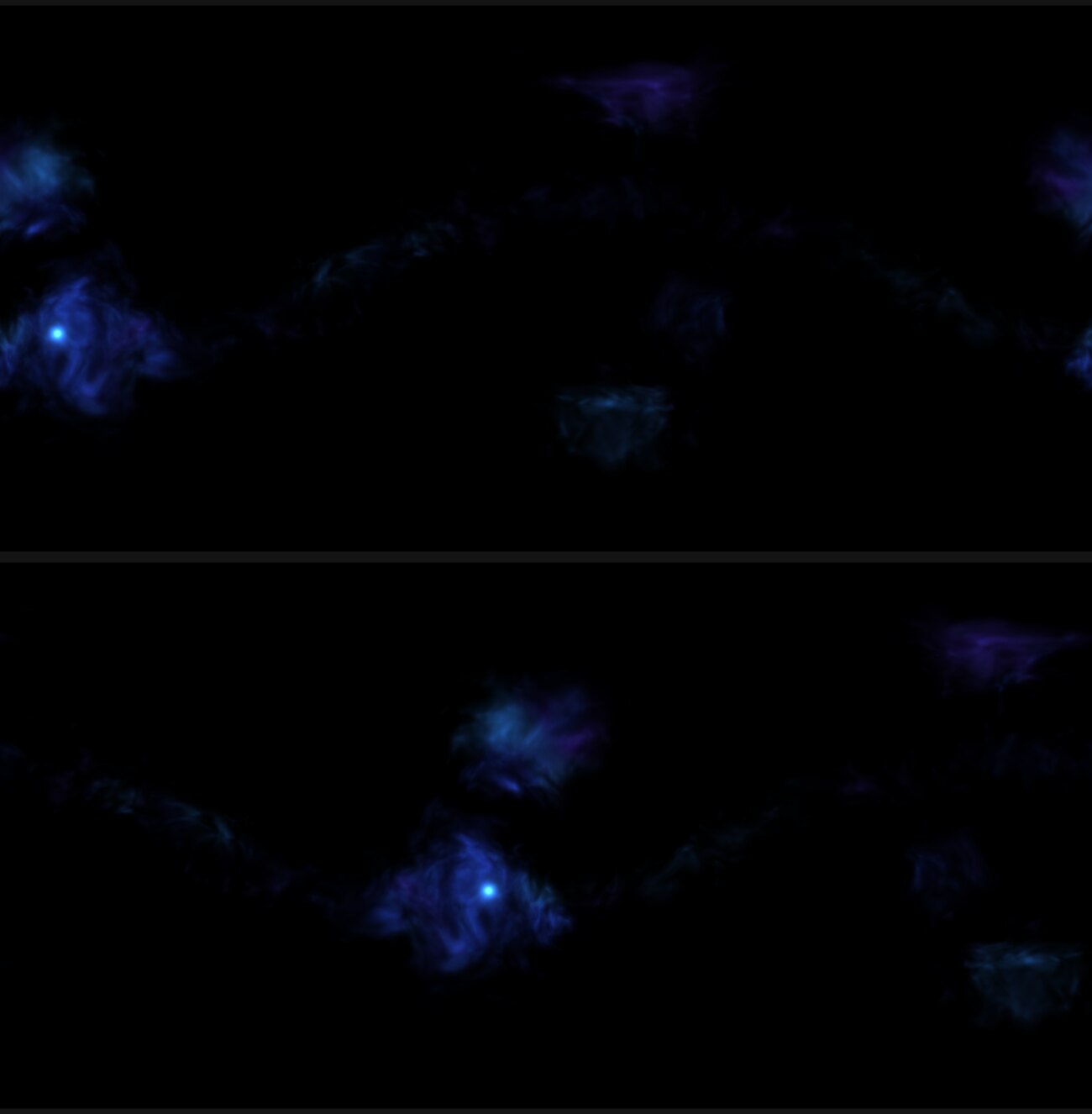Top: the correct inverse. Bottom: the same seed with the sign of z flipped. The belt survives, but the star and every cloud mass moved.

Verify this against your engine’s actual sampling. Memory is not good enough here.

Step 4: decide where gas may exist

The shader builds the nebula in stages. Each stage answers one question, and the first is where gas can exist at all.

That is the structure envelope: a galactic belt plus the cloud masses the composition step placed. This function takes warp and chaos as given. Step 5 explains warp. Step 6 explains chaos.

float structure_envelope(vec3 direction, vec3 warp, float chaos) {
	vec3 bent = normalize(direction + warp * anchor_chaos);
	float lobe = (chaos - 0.5) * anchor_lobing;
	float axis_dot = abs(dot(bent, normalize(band_axis)));
	float belt = exp(-pow(axis_dot / band_half_width, band_sharpness));
	float anchors = 0.0;
	for (int index = 0; index < CLOUD_ANCHOR_COUNT; index++) {
		anchors = max(anchors, anchor_mask(cloud_anchors[index], bent, lobe));
	}
	return clamp(belt * belt_weight + anchors + coverage_bias, 0.0, 1.0);
}

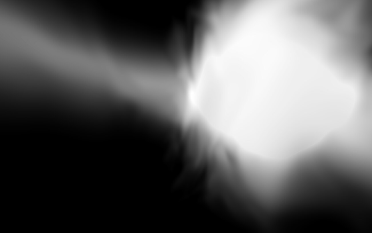The envelope on its own, contrast-stretched. The belt runs across the frame and the bright caps are the cloud masses the composition step placed.

The envelope biases a threshold. Multiply the final colour by it and its outline becomes visible in the image. Bias the density threshold instead and nothing traces it.

The falloff is measured in angle. A ramp written across a span of cosines is narrow near the centre of a spherical cap and vanishes at its edge. For a mass a third of a radian wide that works out to about five degrees, so the anchor behaves as a hard threshold.

// Expressed in angle rather than in cosine, which matters more than it looks.
float anchor_mask(vec4 anchor, vec3 direction, float lobe) {
	float radius = acos(clamp(anchor.w, -1.0, 1.0));
	if (radius < 0.001) {
		return 0.0;   // an anchor switched off carries a cosine above one
	}
	float angle = acos(clamp(dot(direction, normalize(anchor.xyz)), -1.0, 1.0));
	float reach = radius * (1.0 + lobe);
	return 1.0 - smoothstep(reach * ANCHOR_CORE, reach, angle);
}

Working in angle lets the falloff be stated directly: full strength in the core, zero at the nominal radius.

Step 5: let smooth octaves decide the silhouette

The second question is how much gas exists at a given point. The answer contains the most important rule in this shader.

float gas_density(vec3 point, vec3 warp, float envelope, float shells) {
	vec3 fields = cloud_fields(point + warp * 1.25);
	// The boundary is a contour of the smooth field only.
	float level = fields.z + (envelope - 1.0) * gas_falloff;
	float contour = smoothstep(gas_threshold, gas_threshold + gas_softness, level);
	// Detail lives entirely inside that contour, where it can add structure
	// without ever deciding where the gas stops.
	float filament = smoothstep(0.28, 0.78, fields.y);
	float detail = mix(0.34, 1.18, fields.x) * (0.80 + 0.20 * filament);
	return clamp(contour * detail * mix(0.90, 1.10, shells), 0.0, 1.0);
}

fields.z holds only the first three octaves. fields.x and fields.y hold all seven.

The smooth octaves decide the silhouette on their own. Widening the smoothstep is not a substitute. When high-frequency detail determines where the boundary falls, a wider ramp just moves the crossing point, and the edge is equally abrupt there. Removing the detailed octaves from the decision is the only fix.

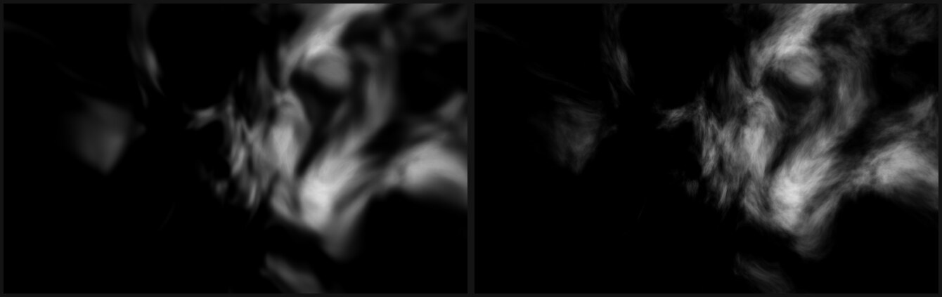The density field, where the difference shows. Left: the contour reads the smooth field, so the outer boundary is soft and the detail sits inside it. Right: the same line reading all seven octaves, which puts high-frequency detail on the boundary itself.

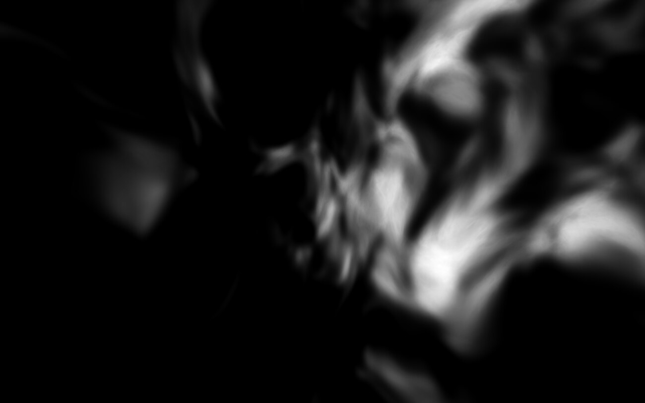Density after the contour decides the edge, contrast-stretched. Detail is everywhere, and none of it decides where the cloud ends.

Every function in steps 4 and 5 reads cloud_fields, which is fractional Brownian motion. It is the same smooth noise summed over seven octaves, each at double the frequency and half the amplitude of the last. Low octaves contribute broad masses, high ones contribute grain, and the sum is the classic cloud texture. It returns three fields from one pass, because each is wanted somewhere and sampling the noise three times over costs three times as much:

// x: plain fBm. y: ridged, for filaments. z: the first LOW_OCTAVES only.
vec3 cloud_fields(vec3 point) {
	vec3 p = point;
	float body = 0.0;
	float body_norm = 0.0;
	float low = 0.0;
	float low_norm = 0.0;
	float ridge = 0.0;
	float ridge_norm = 0.0;
	float body_amplitude = 0.5;
	float ridge_amplitude = 0.5;
	float ridge_gate = 1.0;
	for (int octave = 0; octave < CLOUD_OCTAVES; octave++) {
		float noise = simplex_noise(p);
		body += body_amplitude * (noise * 0.5 + 0.5);
		body_norm += body_amplitude;
		if (octave < LOW_OCTAVES) {
			low += body_amplitude * (noise * 0.5 + 0.5);
			low_norm += body_amplitude;
		}
		float sharpened = 1.0 - abs(noise);
		sharpened *= sharpened;
		ridge += ridge_amplitude * sharpened * ridge_gate;
		ridge_norm += ridge_amplitude;
		ridge_gate = clamp(sharpened * 1.7, 0.0, 1.0);
		p = OCTAVE_TURN * p * 2.07 + vec3(7.1, 3.7, 5.9);
		body_amplitude *= 0.55;
		ridge_amplitude *= 0.55;
	}
	return vec3(body / body_norm, ridge / ridge_norm, low / low_norm);
}

CLOUD_OCTAVES is 7 and LOW_OCTAVES is 3. simplex_noise is smooth gradient noise, the standard Ashima 3D implementation, unmodified. worley_f1 is an ordinary cellular first-distance: the distance to the nearest of a set of scattered points. Thresholded, it gives the gas its shell-like clumping, dark pockets with brighter walls between them.

The ridged channel folds the noise at zero, 1.0 - abs(noise), so every zero crossing becomes a bright crease. Summed over octaves, the creases are the filaments.

One modification between octaves:

// A rotation-and-scale between octaves. Turning the domain as well as scaling it
// stops the octaves from stacking their features onto the same axes. Without it,
// plain fBm looks like grid-aligned mould.
const mat3 OCTAVE_TURN = mat3(
	vec3(0.00, 0.80, 0.60),
	vec3(-0.80, 0.36, -0.48),
	vec3(-0.60, -0.48, 0.64)
);

Domain warping means sampling a field at a position displaced by another noise field. The field itself does not change. The coordinates it is read through bend, and straight features bend with them.

The warp uses its own shorter fBm, three octaves, sampled three times to make a vector:

float smooth_fbm(vec3 point) {
	vec3 p = point;
	float value = 0.0;
	float norm = 0.0;
	float amplitude = 0.5;
	for (int octave = 0; octave < WARP_OCTAVES; octave++) {
		value += amplitude * (simplex_noise(p) * 0.5 + 0.5);
		norm += amplitude;
		p = OCTAVE_TURN * p * 2.11 + vec3(4.3, 8.9, 2.7);
		amplitude *= 0.5;
	}
	return value / norm;
}

vec3 warp_field(vec3 point) {
	return vec3(
		smooth_fbm(point + vec3(1.7, 9.2, 4.3)),
		smooth_fbm(point + vec3(8.3, 2.8, 6.1)),
		smooth_fbm(point + vec3(5.1, 7.4, 1.9))
	) - vec3(0.5);
}

Domain warping then runs at two levels. The second warp bends the first, which produces the long sweeping curl a single warp cannot:

vec3 warp_near = warp_field(direction * 0.40 + seed * 0.09);
vec3 warp_far = warp_field(direction * 0.85 + warp_near * 1.35 + seed.zxy * 0.13);
// Enough warp to curl the folds, and no more. Pushed harder, it stops reading
// as turbulence and starts reading as brush strokes combed in one direction.
vec3 warp = warp_near * 1.10 + warp_far * 0.72;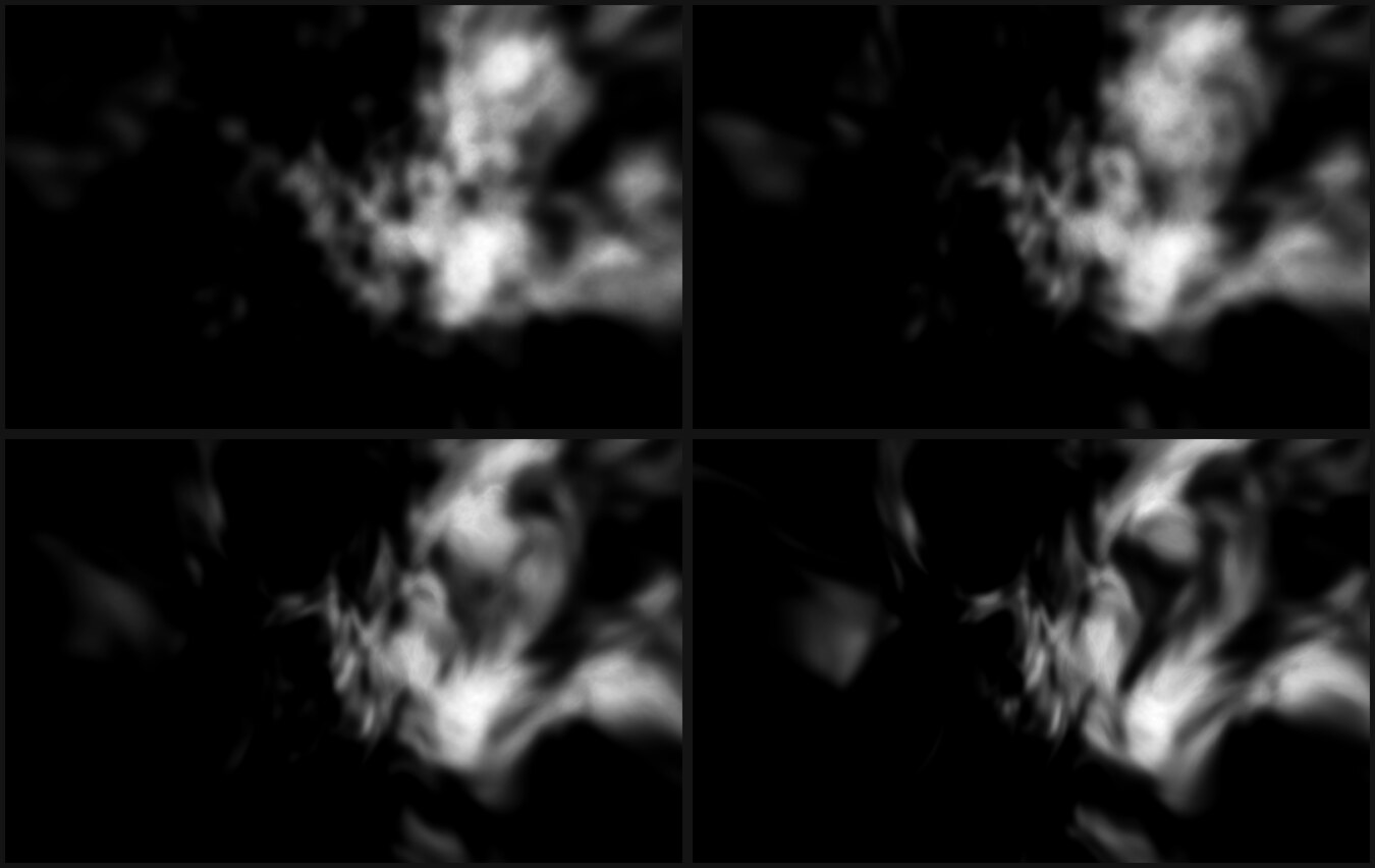

The density field, one base pattern, with the warp scaled to 0, 0.35, 0.7 and 1.0. Reading left to right and top to bottom, the same masses stretch and curl into filaments.

Step 6: assemble the fields, then march them

The pieces described so far are functions. This is the order fragment() calls them in, which is not obvious from any of them alone.

Four details in this block are critical for the final shape:

• chaos feeds the envelope, so the size of each mass varies.
• region scales the envelope afterwards, giving dense and thin areas rather than one uniform opacity.
• corridor suppresses gas in long coherent stretches.
• All three read .z, the smooth channel, for the reason step 5 gives.

vec3 seed = seed_offset * 0.19;
vec3 star_axis = normalize(star_direction);

vec3 warp_near = warp_field(direction * 0.40 + seed * 0.09);
vec3 warp_far = warp_field(direction * 0.85 + warp_near * 1.35 + seed.zxy * 0.13);
vec3 warp = warp_near * 1.10 + warp_far * 0.72;

// Smooth octaves only. Taking these from the detailed output punches
// fractal-edged holes through the gas, which is the step 5 mistake one stage on.
float region = cloud_fields(direction * 0.38 + warp * 0.60 + seed * 0.17).z;
float chaos = cloud_fields(direction * 1.35 + warp * 0.95 + seed.zyx * 0.21).z;
float structure = structure_envelope(direction, warp, chaos);

// Void corridors: very low frequency, smooth over tens of degrees. Applied to
// the envelope rather than the colour, so gas thins toward them.
float corridor = cloud_fields(direction * 0.23 + seed.yzx * 0.13 + warp * 0.22).z;
structure *= mix(1.0 - void_depth, 1.0, smoothstep(0.30, 0.72, corridor));
structure = clamp(structure * mix(0.68, 1.22, region), 0.0, 1.0);

float shells = smoothstep(0.30, 0.86, worley_f1(direction * 1.15 + warp * 1.1 + seed * 0.11));

// Two low-frequency fields distribute the palette, read off the warp already paid for.
float hue_field = clamp(0.5 + warp_far.y * 3.0, 0.0, 1.0);
float accent_field = clamp(0.5 + warp_near.z * 3.2, 0.0, 1.0);
float accent_region = smoothstep(0.60, 0.88, accent_field);

Ray marching is integration by sampling: walk along the view ray in fixed steps, evaluate the density at each, and accumulate what each step emits.

Sixteen steps here, accumulated front to back and attenuated by Beer-Lambert transmittance. Transmittance dims everything behind each sample by an exponential of the density that sample adds. That is what lets near gas veil far gas.

The interval is the same for every direction, so this integrates a 3D field to give the sky thickness. No depth is traced through a scene. The march is skipped where the envelope is negligible.

vec3 accumulated = vec3(0.0);
float transmittance = 1.0;
float column = 0.0;   // total gas, kept apart from transmittance for the star

if (structure > MARCH_CUTOFF) {
	for (int layer = 0; layer < MARCH_STEPS; layer++) {
		float depth = (float(layer) + 0.5) / float(MARCH_STEPS);
		vec3 sample_position = direction * (0.85 + depth * 3.60) + seed * 0.23;
		float density = gas_density(sample_position, warp, structure, shells);
		column += density;
		if (density <= 0.001) {
			continue;
		}
		float toward_light = gas_density(
			sample_position + star_axis * 0.30, warp, structure, shells
		);
		float lit = clamp(0.16 + (density - toward_light) * 2.2 + depth * 0.08, 0.0, 1.0);

		vec3 tone = mix(gas_body, gas_secondary, smoothstep(0.28, 0.80, hue_field));
		tone = mix(tone, gas_accent, accent_region * 0.72);
		vec3 layer_colour = mix(gas_shadow, tone, smoothstep(0.02, 0.26, density));
		layer_colour = mix(layer_colour, gas_light, smoothstep(0.72, 1.0, lit) * 0.10);
		// The only term that exceeds 1.0, and therefore the only thing that blooms.
		vec3 core_colour = mix(tone, gas_light, 0.28);
		layer_colour += core_colour * pow(density, 4.0) * core_energy * lit;

		float emission = pow(density, EMISSION_EXPONENT);
		accumulated += transmittance * layer_colour * emission * 0.42 * nebula_energy;
		transmittance *= exp(-density * 0.13);
	}
}

Most of the result comes from three lines: the two that build emission and accumulated, and the one that decays transmittance.

Emission rises faster than density. Recombination, which is ions recapturing electrons and emitting as they do, scales near-square with density, because it needs the two to meet. The exponent used here is 1.85. This is the main difference between gas that glows and gas that looks like an evenly lit solid. Linear emission averaged over sixteen samples produces one flat mid tone across the whole cloud, which looks like milk. At 1.85 the same field gives faint envelopes over most of the volume and a few bright knots, and that distribution looks luminous.

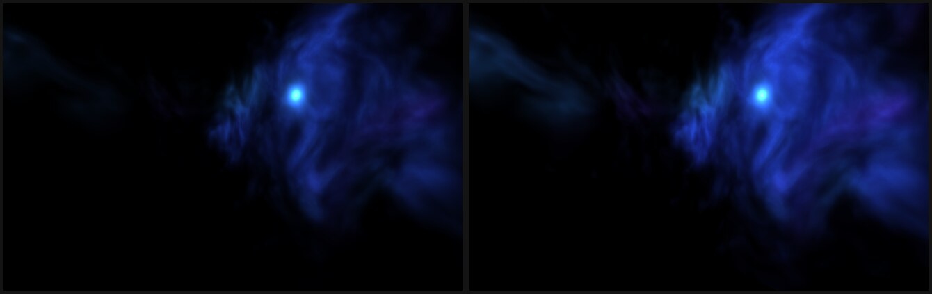The frame the camera actually sees. Left: exponent 1.85. Right: the same sky at 1.0, where every sample contributes in proportion, the average flattens, and the cloud becomes an evenly lit haze.

The 0.13 extinction coefficient is deliberately small, because emitting gas is optically thin. It glows through its own depth and stars remain visible behind it. Increasing it enough to occlude turns the cloud into a surface regardless of its colour.

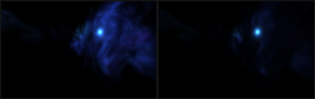Left: extinction 0.13. Right: the same sky at 1.30, where the medium hides its own depth and the glow never accumulates.

Lighting uses a density gradient in place of light transport. The march takes a second density sample toward the star and compares the two:

float toward_light = gas_density(sample_position + star_axis * 0.30, warp, structure, shells);
// Positive where this sample is less buried than its neighbour
// toward the star, so edges facing the star catch the light.
float lit = clamp(0.16 + (density - toward_light) * 2.2 + depth * 0.08, 0.0, 1.0);

Occlusion comes from a separate, nearer dust layer that only subtracts:

float dust_field = cloud_fields(direction * 0.60 + warp * 1.25 + seed.yzx * 0.31).z;
float dust = smoothstep(0.46, 0.98, dust_field) * structure * dust_strength;
colour *= exp(-dust);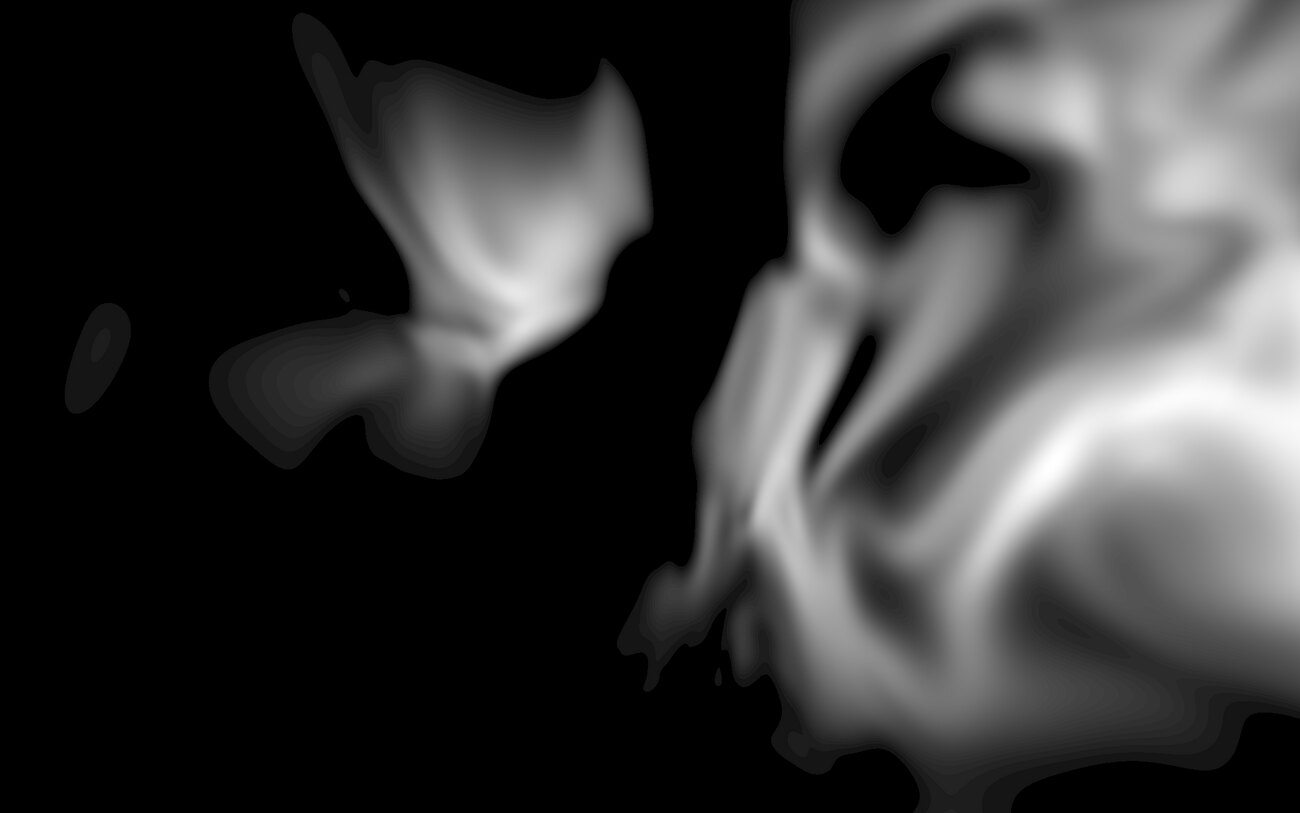

The dust field, contrast-stretched. It never emits. It only subtracts light from whatever is behind it.

Step 7: put the star inside the picture

Compositing the star over the finished image makes it read as a lens flare rather than as part of the scene. The difference is whether gas crossing the star attenuates it.

The march accumulates total gas along the ray separately from transmittance. The star is then attenuated by that column:

float star_occlusion = exp(-column * star_extinction - dust * 1.4);

Star colour also has to survive at the bright end. At the intensity needed to light the halo, every star clips to white, so a red dwarf looks identical to a blue giant. Normalising to the brightest channel first lets the clamp reduce brightness without shifting hue:

vec3 disc_hue = star_colour / max(max(star_colour.r, star_colour.g), max(star_colour.b, 1e-4));
colour += disc_hue * min(star_intensity, star_disc_peak) * disc * star_occlusion;

Light absorbed by the medium is also scattered. Re-emitting it in proportion to the amount absorbed places the glow inside the cloud. The glow then follows the gas structure, and no clean radial gradient appears over it:

vec3 scatter_tint = mix(star_colour, gas_light, 0.45);
float scattered = (1.0 - star_occlusion) * (glare * 0.011 + bloom_seat * 0.00042);
colour += scatter_tint * star_intensity * scattered * star_scatter;

Step 8: two post-processing lines, one for colour and one for edges

Even with a correct march, the visual result can fail in two specific ways.

The first is desaturation. Emission lines are narrow, so a real nebula is far more saturated than a sum of tinted translucent layers. Averaging many samples pulls every hue toward the grey axis, and the result comes out cream. The fix is to restore saturation afterwards and then renormalise. The second half is easy to omit:

float luma = dot(colour, vec3(0.2126, 0.7152, 0.0722));
vec3 saturated = max(mix(vec3(luma), colour, gas_saturation), vec3(0.0));
// Renormalised back to the luminance it started with. Pushing chroma past
// the gamut drives channels negative, and clamping them there quietly
// darkens every dim, near-neutral pixel.
float saturated_luma = dot(saturated, vec3(0.2126, 0.7152, 0.0722));
vec3 colour_out = saturated * (luma / max(saturated_luma, 1e-5));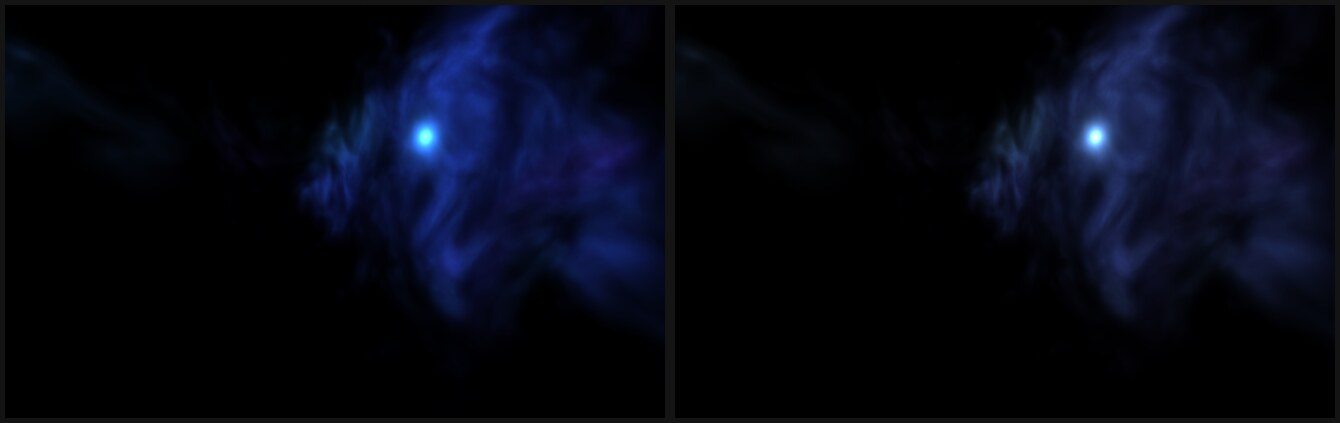

Left: saturation restored and renormalised. Right: the same frame straight out of the integral, pulled toward grey.

The second is the cloud boundary. Every generator described so far leaves a long dim tail. A tail one or two levels above zero covers the frame in something that looks like a dirty lens. The tail has to go.

Subtracting a floor is the obvious way to remove it, and the wrong one. It cuts the tail at a hard contour. That contour lands exactly where the cloud is dissolving, so the edge ends up looking cut out of paper.

A smoothstep knee reaches the same true black with nothing visible at the boundary:

colour_out *= smoothstep(0.0, black_floor * 5.0, luma);

The floor is 0.00012. That value looks low until you account for sRGB encoding. A linear floor of a few thousandths removes everything up to about a tenth of perceived brightness. That is the entire range over which a cloud fades out.

Step 9: bake only the reachable patch

The nebula does not move, so it is rendered once into a texture and the shader never runs again. The remaining question is the texture’s shape.

An equirectangular sphere spreads its texels evenly across directions the camera cannot reach. Take 4096x2048, which is a reasonable size to reach for: it carries 11.4 pixels per degree. A 1920 wide frame across a 74 degree horizontal field needs 25.9. Such a texture is magnified 2.3 times in the only region that is visible, and six sevenths of it is never sampled.

Matching screen density with a sphere is not practical:

Screen	Sphere at screen density	Cone at screen density
1920x1080	9331x4665, 249 MB	2613x1664, 25 MB
2560x1440	12441x6220, 443 MB	3483x2219, 44 MB
3840x2160	18661x9331, 996 MB	5225x3328, 100 MB
5120x2880	24882x12441, 1.73 GB	6967x4437, 177 MB

Every size in this section is RGBH, which is three 16-bit floats and 6 bytes per texel, with no mipmaps. Multiply width by height by six to get any of them.

The cone the camera can reach spans about 101 by 64 degrees. That is the wider of the two compositions, plus the camera’s travel, plus margin. At 2560x1600 it holds one texel per screen pixel at 1080p.

That is 25.4 pixels per degree against the 25.9 a 1080p frame asks for. The shipped 2560x1600 sits a little under the table’s calculated 2613x1664, which is why it costs 23 MB against the table’s 25.

Read it against the first row of that table. A sphere reaching the same density costs 249 MB. At equal quality the cone is a tenth of the memory.

Rendering it is a SubViewport with a full-size ColorRect, one frame, then the image read back:

func bake(identity: SkyboxIdentity, texture_size: Vector2i, cone: bool) -> Texture2D:
	var viewport := SubViewport.new()
	viewport.size = texture_size
	viewport.use_hdr_2d = true          # the core term exceeds 1.0
	viewport.render_target_clear_mode = SubViewport.CLEAR_MODE_ONCE
	viewport.render_target_update_mode = SubViewport.UPDATE_ONCE
	add_child(viewport)

	var target := ColorRect.new()
	target.size = Vector2(texture_size)
	var material := ShaderMaterial.new()
	material.shader = SKYBOX_SHADER
	var look := SkyboxLook.from(identity)
	material.set_shader_parameter(&"seed_offset", identity.shader_offset())
	material.set_shader_parameter(&"band_axis", identity.band_axis())
	material.set_shader_parameter(&"cloud_anchors", identity.cloud_anchors())
	material.set_shader_parameter(&"star_direction", identity.star_direction())
	material.set_shader_parameter(&"gas_body", look.gas_body)
	# ... the rest of the identity and the look, one uniform each
	material.set_shader_parameter(&"projection", 1 if cone else 0)
	if cone:
		material.set_shader_parameter(&"cone_basis", cone_basis())
		material.set_shader_parameter(
			&"cone_tan", Vector2(tan(CONE_HALF_ANGLES.x), tan(CONE_HALF_ANGLES.y))
		)
	target.material = material
	viewport.add_child(target)

	await RenderingServer.frame_post_draw

	var image := viewport.get_texture().get_image()
	viewport.queue_free()
	return ImageTexture.create_from_image(image)

use_hdr_2d is required. The glow pass only reads values above 1.0, so an 8-bit target clamps away the core term. That term is the only thing in the frame that blooms.

The basis the cone is written along, which the sky shader reads back:

static func cone_basis() -> Basis:
	var forward := SkyboxIdentity.VIEW_DIRECTION.normalized()
	var right := forward.cross(Vector3.UP)
	if right.length_squared() < 0.0001:
		right = forward.cross(Vector3.RIGHT)
	right = right.normalized()
	var up := right.cross(forward).normalized()
	return Basis(right, up, forward)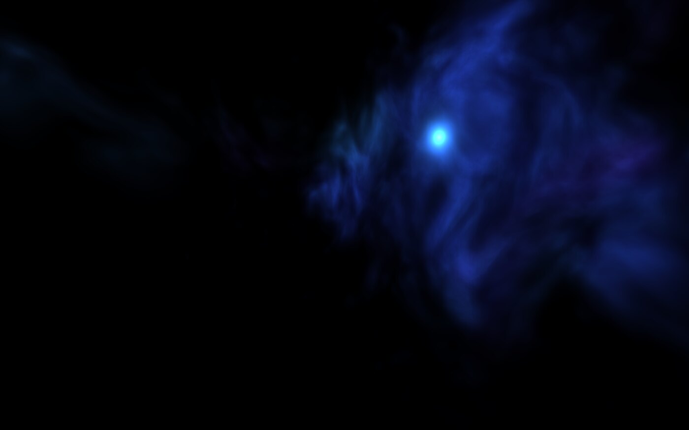

The shipped texture. Not a map of a sphere. A window onto the patch of sky the camera can turn to.

The same seed as a full equirectangular sphere, for comparison. Most of it is never sampled:

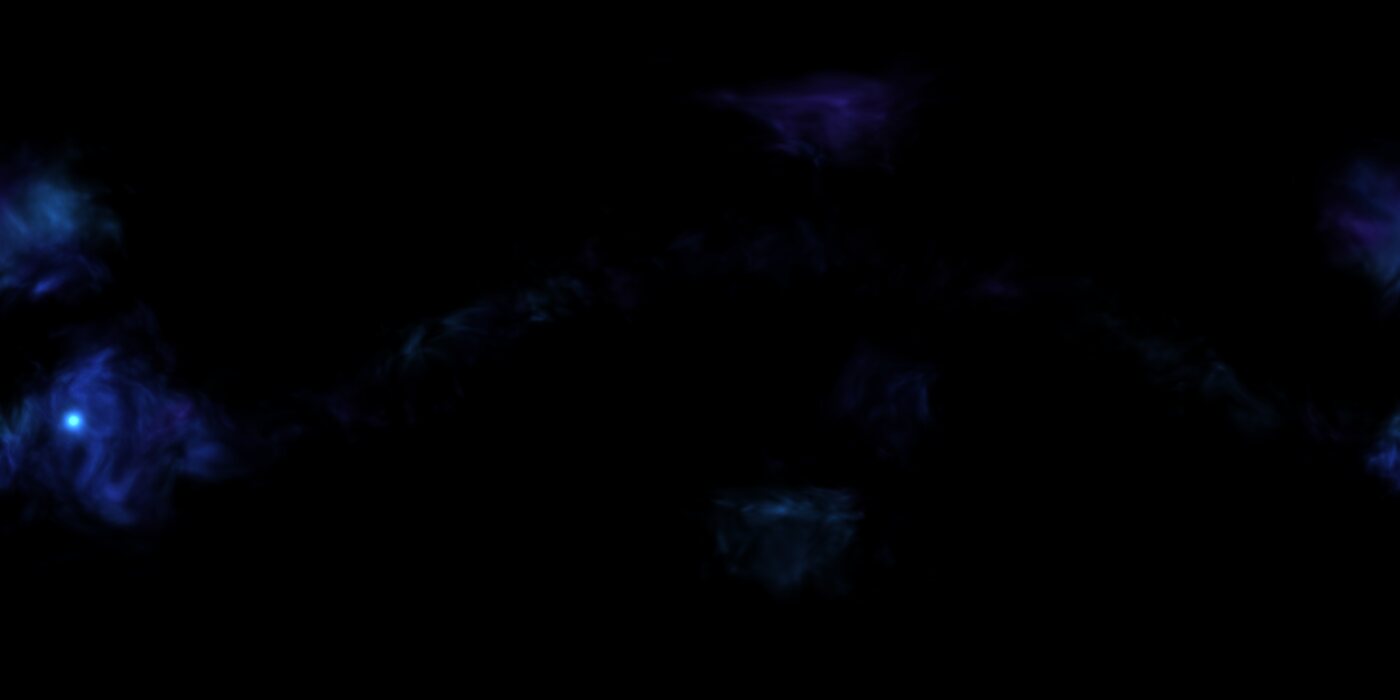The equirectangular version. The camera reaches about a seventh of it.

PanoramaSkyMaterial expects a full sphere and cannot draw a cone. A custom sky shader can, by projecting the eye direction back through the bake’s own projection:

void sky() {
	// A sky processor may not return early, so the whole lookup is one
	// expression guarded by a mask rather than a chain of exits.
	vec3 direction = normalize(EYEDIR);
	float forward = dot(direction, cone_forward);
	float safe_forward = max(forward, 0.0001);
	vec2 plane = vec2(dot(direction, cone_right), dot(direction, cone_up)) / safe_forward;
	vec2 ndc = plane / cone_tan;
	vec2 uv = vec2(ndc.x, -ndc.y) * 0.5 + 0.5;
	float reach = max(abs(ndc.x), abs(ndc.y));
	float inside = step(0.0, forward) * (1.0 - smoothstep(1.0 - cone_feather, 1.0, reach));
	COLOR = texture(cone_panorama, clamp(uv, vec2(0.0), vec2(1.0))).rgb * inside;
}

Outside the cone it returns black. The camera cannot point there, so that is the correct value.

Godot sky shaders have two properties that fail silently:

A sky processor cannot use return. An early exit fails to compile silently. The sky renders black while the star billboards still draw over it, which looks like a sampling bug. That is why the lookup uses a mask throughout.

A mipmapped sampler in a sky shader has no useful derivatives. A sampler picks its mip level from the screen-space derivatives of the UV, which is how fast the coordinate changes between neighbouring pixels. A sky shader has none worth reading, so the sampler falls to the smallest mip and returns the average of a mostly black image. That failure is silent too. filter_linear fixes it, and the bake already matches screen density, so there is nothing to filter.

Step 10: why the stars are geometry

The cone bake holds 25.4 pixels per degree, which is enough to keep a point sharp at 1080p. So a texture can hold the stars, and geometry is still the better answer.

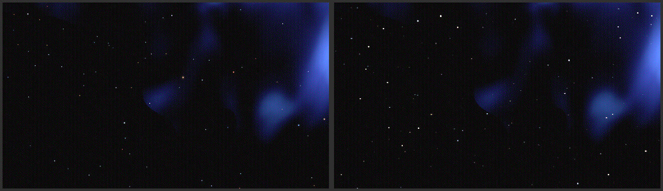One-to-one crops, brightened. Left: billboards. Right: the same stars written into the cone bake. Sharpness remains better than expected at this density, and the bake flattens the colour spread and the brightness peaks the billboard layer draws for itself.

The nebula and the stars are different kinds of signal.

A nebula is low frequency. Magnify it 2.3 times and nothing in it is destroyed, because it contains no feature a soft pixel can lose. Its bake resolution is a knob for quality. An inaccurate choice costs sharpness and nothing else.

A star is the highest frequency content an image can carry. It is a single point, and any magnification turns it into a disc.

The two want different things from a texture, and one resolution cannot satisfy both. Bake the content that tolerates softness, and draw the content that does not as geometry, which has no fixed resolution.

The table in step 9 states the same argument numerically. Keeping stars sharp in the texture means re-baking per display: 25 MB at 1080p, 44 at 1440p, 100 at 4K, 177 at 5K. Billboards cost 1622 instances (1600 faint stars, 12 bright stars, 10 galaxies) and one draw call at every resolution. They stay sharp at all of them.

Bright stars have a second reason. They carry halos, and a halo must respond to the glow pass at its actual on-screen size, which a baked one cannot do.

Drawing only the stars the camera can reach

The same cone logic applies to the billboards, and more strongly. These are scene geometry. A star outside the frame never reaches the sky texture. It also never reaches the radiance map, the blurred copy of the sky the engine lights the scene with. It contributes nothing, and is still submitted, culled and discarded every frame.

## Half-angle of the cone the star layers are drawn into.
##
## **A star outside the frame reaches nothing.** These are scene billboards. They
## are not part of the sky texture, so they never enter the radiance map either.
## A star the camera cannot turn to is work with no output at all.
const _STAR_CONE := 0.95

Sampling that cone evenly requires one detail. A uniform draw on the angle crowds the centre of the frame. The area of a cap grows with the cosine, so a draw uniform in the cosine is uniform per unit of sky:

func _sphere_direction(rng: RandomNumberGenerator) -> Vector3:
	var cosine := lerpf(cos(_STAR_CONE), 1.0, rng.randf())
	var angle := acos(clampf(cosine, -1.0, 1.0))
	var azimuth := rng.randf() * TAU
	return SkyboxIdentity.direction_near_at(SkyboxIdentity.VIEW_DIRECTION, angle, azimuth)

Half the field clusters on the galactic belt. The belt is a great circle and the cone is a spherical cap, so they overlap along part of the circle only. Rejection sampling finds that part: draw on the belt, keep the draw if it lands inside the cone, try again if it does not.

Instance counts then drop to hold the same on-screen density. Both configurations were measured by unprojecting every instance against a 1920x1080 frame:

Placement	Instances	In frame	Wasted
Spread over the sphere	6086	762	87%
Confined to the cone	1622	783	52%

Same visual result, 73 per cent fewer instances. The remaining 52 per cent is the rotation margin, which step 12 uses.

One more detail about the field, unrelated to the cone. The brightness distribution matters more than the count:

# A log draw is what makes a dim star ordinary and a brilliant one rare. A
# uniform draw gives every star the same claim on the eye.
var luminosity := clampf(-log(maxf(1.0 - rng.randf(), 1e-6)) / 6.0, 0.0, 1.0)
var scale := base_size * (0.55 + pow(luminosity, 2.2) * 2.4)

The material is additive, so overlapping stars sum, and billboarded, so the quad turns to face the camera. The sprite’s transparent surround leaves the gas behind it alone:

material.albedo_texture = sprite
material.vertex_color_use_as_albedo = true
material.shading_mode = BaseMaterial3D.SHADING_MODE_UNSHADED
material.transparency = BaseMaterial3D.TRANSPARENCY_ALPHA
material.blend_mode = BaseMaterial3D.BLEND_MODE_ADD
material.billboard_mode = BaseMaterial3D.BILLBOARD_ENABLED
material.billboard_keep_scale = true
material.no_depth_test = true

And one failure mode worth knowing, because the symptom is hard to diagnose:

# The shell is far outside anything else in the scene. Without this, the layer
# culls the moment the bounds of the camera do not reach it.
layer.custom_aabb = AABB(Vector3.ONE * -_STAR_SHELL * 1.2, Vector3.ONE * _STAR_SHELL * 2.4)

A MultiMeshInstance3D computes its bounds lazily. Without an explicit custom_aabb, the entire star field disappears at certain camera angles.

Step 11: light the scene from the sky

The sky is also the only light source in the scene. Anything drawn in front of it is lit by the star this seed generated, in the colours this seed selected.

var look := SkyboxLook.from(skybox_identity)
var body := look.gas_body
var accent := look.gas_accent
var stellar := skybox_identity.stellar.light_color
_world_environment.environment.ambient_light_color = (
	body.lerp(accent, 0.18).lerp(stellar, 0.24).lightened(0.10)
)
key.light_color = stellar.lightened(0.08)
_aim_at_star(key)

Aiming the key light directly at the star is physically correct and leaves the subject backlit and unreadable. The aim blends part of the way back toward the viewer:

## The blend keeps the light arriving from the side of the frame the star is on.
## It still puts some of that light on the faces the player looks at.
var aim := toward_star.normalized().lerp(toward_viewer, _STAR_KEY_FILL).normalized()

Step 12: move the camera, slowly

A completely static frame looks painted. Fixing that needs no new machinery. The camera can already turn and the composition already reserves the room, so an idle drift costs two sine waves.

## Seconds per sweep, one per axis. They are deliberately not multiples of each
## other, so the pair does not visibly return to where it started.
const _DRIFT_YAW_PERIOD := 47.0
const _DRIFT_PITCH_PERIOD := 31.0

func _drift_camera() -> void:
	var yaw := (
		sin(_elapsed * TAU / _DRIFT_YAW_PERIOD) * SkyboxIdentity.MAX_VIEW_YAW * _DRIFT_SHARE
	)
	var pitch := (
		sin(_elapsed * TAU / _DRIFT_PITCH_PERIOD) * SkyboxIdentity.MAX_VIEW_PITCH * _DRIFT_SHARE
	)
	aim_camera(yaw, pitch)

The periods are not multiples of each other, so the pair takes about twenty minutes to repeat. The drift also uses only part of the cone, leaving room for player-driven camera movement.

The camera pivots about the origin, so it keeps looking at the centre of the composition at any angle. Values outside the cone clamp:

func aim_camera(yaw: float, pitch: float) -> void:
	var clamped_yaw := clampf(yaw, -SkyboxIdentity.MAX_VIEW_YAW, SkyboxIdentity.MAX_VIEW_YAW)
	var clamped_pitch := clampf(
		pitch, -SkyboxIdentity.MAX_VIEW_PITCH, SkyboxIdentity.MAX_VIEW_PITCH
	)
	var base := _MENU_CAMERA if composition == Composition.MENU else _CAMPAIGN_CAMERA
	var turned := base.rotated(Vector3.UP, clamped_yaw)
	var right := turned.cross(Vector3.UP)
	if right.length_squared() > 0.0001:
		turned = turned.rotated(right.normalized(), -clamped_pitch)
	camera.position = turned
	camera.look_at(Vector3.ZERO, Vector3.UP)

One seed and one bake, at minus eight degrees, zero, and plus eight. The bright side holds its corner at every angle.

Because the camera is always moving, every constraint the composition sets has to hold across the whole sweep. The test samples the whole cone: forty seeds by forty-nine angles, checking the star against the screen-right axis of each rotated frame:

var frame_right := axis.cross(Vector3.UP).normalized()
assert_gt(
	star.dot(frame_right),
	0.0,
	"star crossed to the dark side of the frame at yaw %f pitch %f" % [yaw, pitch]
)

The worst case across that sweep clears zero by 0.022.

The diagnostic switch

On a shader like this, build it first.

The shader carries a debug_term uniform that replaces the output with one isolated stage:

if (debug_term == 1) {
	colour_out = vec3(structure);
} else if (debug_term == 2) {
	colour_out = vec3(region);
} else if (debug_term == 3) {
	colour_out = vec3(dust);
} else if (debug_term == 4) {
	colour_out = vec3(brightness_field);
} else if (debug_term == 5) {
	colour_out = vec3(gas_density(direction * 2.0 + seed * 0.23, warp, structure, shells));
}

With a matching entry point on the baker:

## Diagnostic bake that isolates one shader term. Not used by the game.
func bake_debug(identity: SkyboxIdentity, texture_size: Vector2i, term: int) -> Texture2D:
	debug_term = term
	var texture: Texture2D = await bake(identity, texture_size)
	debug_term = 0
	return texture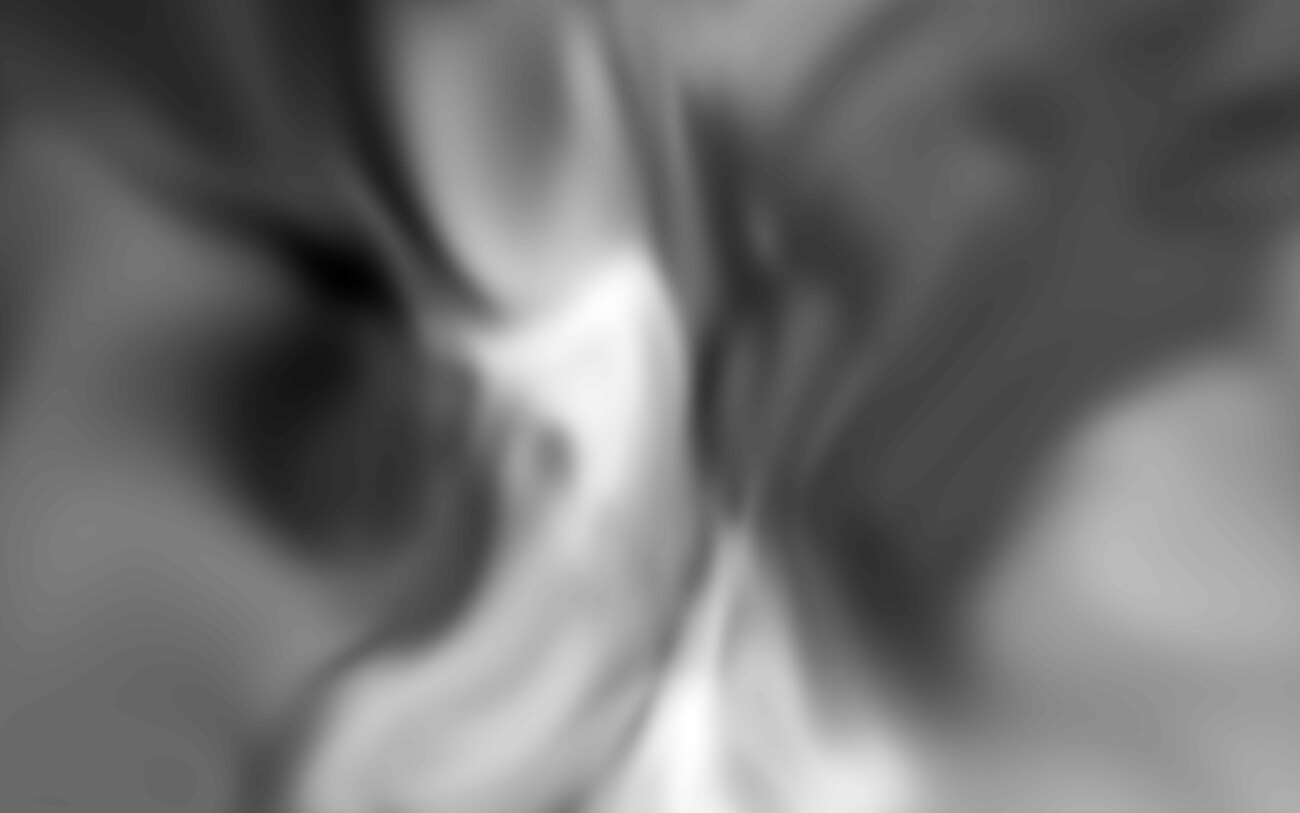

A low-frequency field, contrast-stretched, that varies gas density from place to place. Without it the belt is one even ribbon.

Most of the fixes described in this article came from that switch. A composite of seven fields cannot be debugged by looking at the composite. The hard-edge problem was invisible in the final image and obvious in the envelope on its own.

Results

The seed selects the stellar family, which drives both the star and the five colour roles of the gas. Same code, four seeds:

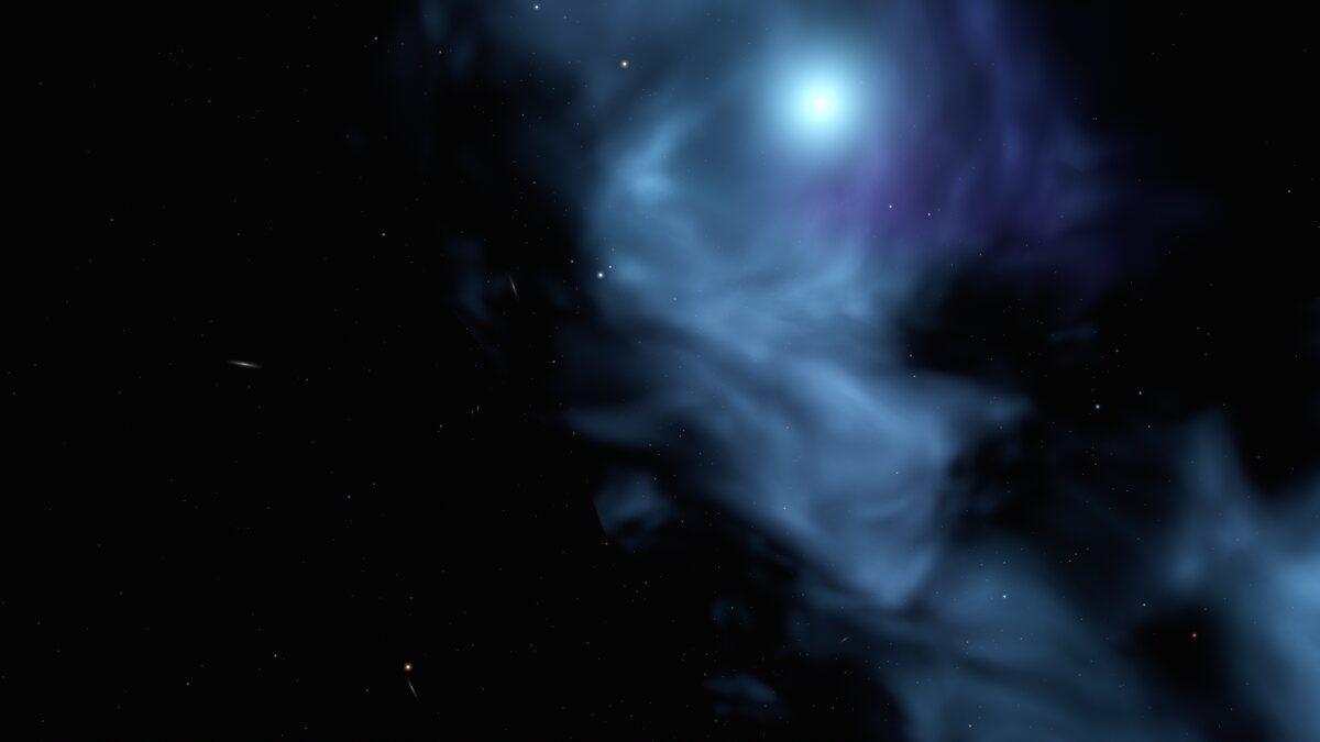Blue giant. Tight, bright and dusty. Hot stars carve their neighbourhood.

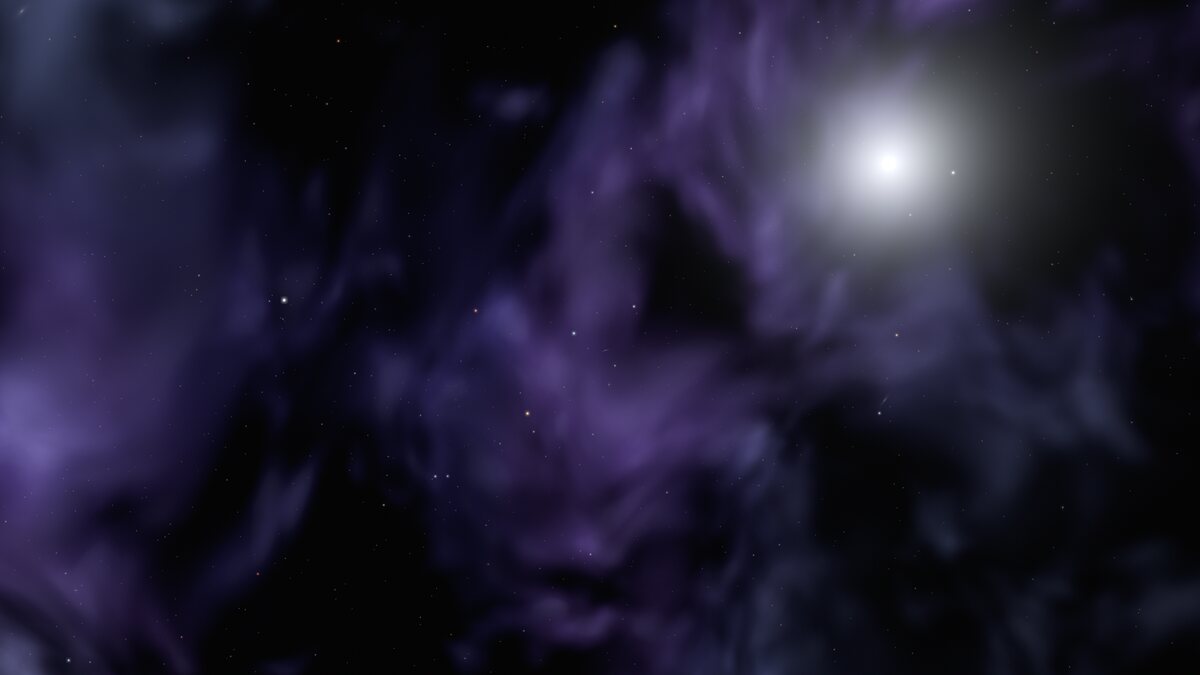A white star over a wider, cooler belt.

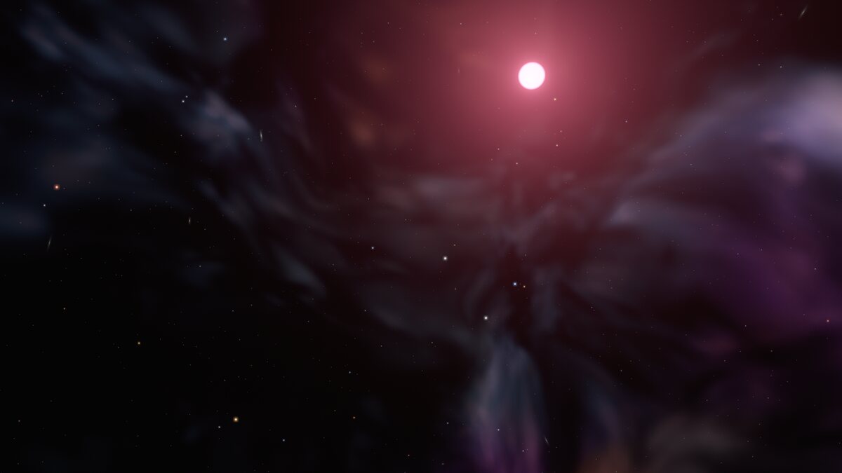Red dwarf. A large dim disc, and warm secondary gas.

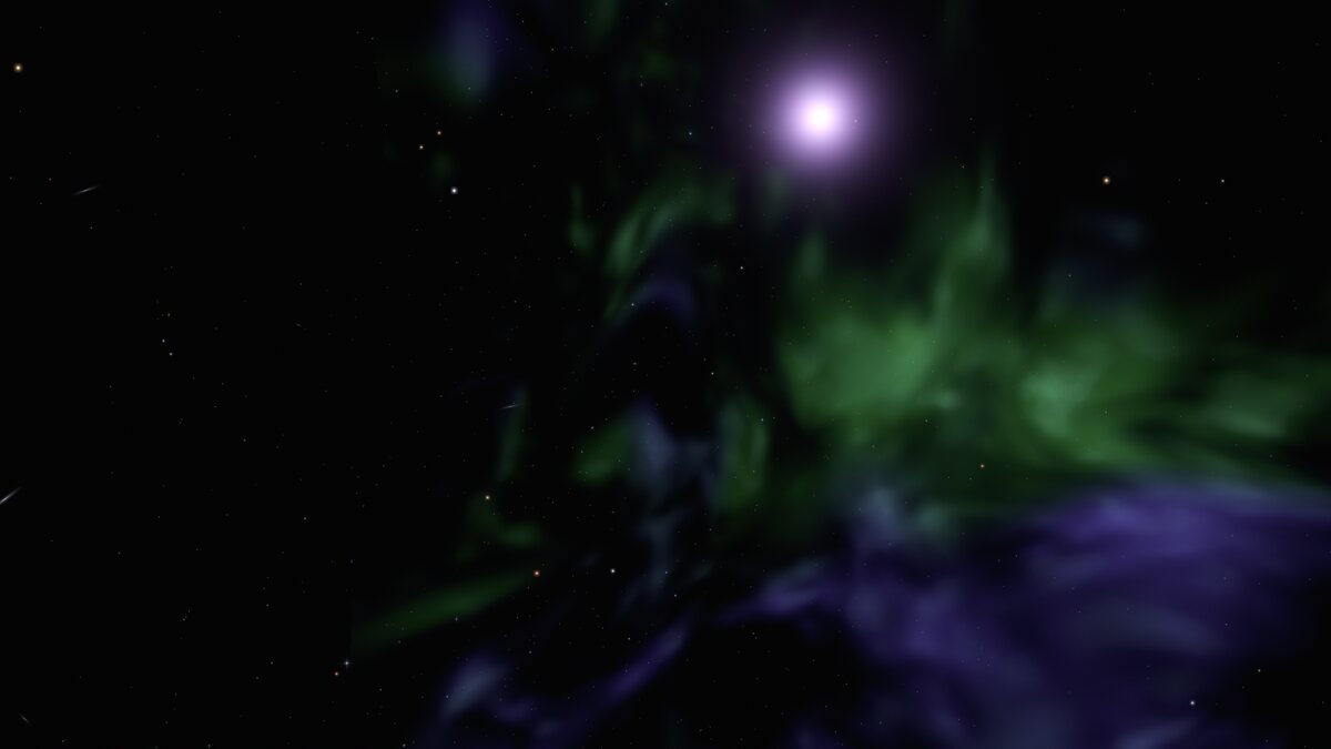The exotic family. It is the only one allowed the sickly green of the setting, and only in its secondary role.

The shadow and main gas stay deep indigo across every family. The star’s temperature is expressed only in the secondary cloud, the accents and the hot edges. The sky never warms into the colours of an active stellar nursery.

One bake costs a single render pass: the viewport renders once and the image is read back. Every scene transition rebakes.

Summary

The goal was to replace FTL’s painters with a generator. I expected the shader to be the painter. It turned out to be closer to the brush, and the painter is the composition stage. A subject holding one side of the frame, dark ground on the other, a star that keeps to its side through every angle the camera can turn. By the time the shader runs, the composition stage already decided everything that makes a sky this sky. That decision is plain integer arithmetic a unit test can hold still.

The same two ideas kept resurfacing under different names. Compose for the camera: the reachable cone shaped the texture, the star field, and the memory budget. And let the smooth fields decide: the silhouette, the regions and the corridors all read the low octaves, while detail only decorates what they chose.

What comes out is one sky per seed, cheap enough to rebake on every scene transition and never store.